3.2. Sizing a heat pump
Sizing a heat pump accurately to ensure we meet the heat load of the house at the design outside temperature (DOT) is important for efficiency and system longevity.
The Coefficient of Performance (COP) is a measure of the efficiency of a heating or cooling system at the moment of calculation, and is defined as the ratio of useful heat or cooling output to the energy input. A higher COP indicates a more efficient system and less running costs for the customer.
Both the COP and the effective output of a heat pump are influenced by several factors. These include the flow temperature of the heat delivery medium in the heating circuit and the outdoor air temperature which affects how easily the latent heat contained in the air is absorbed by the evaporator’s fins and pipework.
For a ground source heat pump, the temperature of the thermal transfer fluid in the brine circuit is equally important as this fluid absorbs heat as it passes through the ground pipework, borehole or collector before releasing it into the evaporator.
Manufacturer data tables
Understanding manufacturer’s data tables is an important part of the process of sizing a heat pump. Each manufacturer displays their output data differently. Care is needed when comparing heat pumps as some technologies, including different refrigerants, can change a heat pump’s performance characteristics. It can also be the case that a heat pump with the model number 16 may not be able to produce 16KW at the DOT for your project’s location.
For example, the table below shows several different DOTs with the respective power outputs for each model listed in the first column. This is particularly helpful as a number of the DOTs for the UK are represented here allowing you to confidently select the unit that provides sufficient heat energy to meet the demand you calculated earlier.
| 35°C flow | 40°C flow | 45°C flow | 50°C flow | 55°C flow | |||||||
|---|---|---|---|---|---|---|---|---|---|---|---|
| Output | SCOP | Output | SCOP | Output | SCOP | Output | SCOP | Output | SCOP | ||
| 3.5kW | -5°C | 4.2 | 4.41 | 4.1 | 4.03 | 4 | 3.65 | 3.9 | 3.37 | 3.8 | 3.1 |
| -3°C | 4.6 | 4.4 | 4.3 | 4.2 | 4 | ||||||
| 0°C | 4.7 | 4.7 | 4.6 | 4.5 | 4.4 | ||||||
| 2°C | 4.9 | 4.9 | 4.9 | 4.7 | 4.6 | ||||||
| 5kW | -5°C | 6.3 | 4.48 | 6 | 4.13 | 5.6 | 3.77 | 5.5 | 3.41 | 5.4 | 3.06 |
| -3°C | 6.8 | 6.4 | 6.1 | 5.9 | 5.8 | ||||||
| 0°C | 6.9 | 6.7 | 6.6 | 6.4 | 6.2 | ||||||
| 2°C | 7.1 | 7 | 6.9 | 6.7 | 6.5 | ||||||
| 7kW | -5°C | 8.2 | 4.36 | 8.1 | 4.13 | 8 | 3.91 | 7.5 | 3.65 | 7 | 3.39 |
| -3°C | 8.8 | 8.6 | 8.4 | 7.9 | 7.4 | ||||||
| 0°C | 9.5 | 9.3 | 9.1 | 8.6 | 8.1 | ||||||
| 2°C | 10 | 9.8 | 9.6 | 9 | 8.5 | ||||||
| 10kW | -5°C | 9.9 | 5.03 | 9.7 | 4.58 | 9.4 | 4.13 | 9.1 | 3.85 | 8.8 | 3.58 |
| -3°C | 10.7 | 10.3 | 10 | 9.6 | 9.2 | ||||||
| 0°C | 11.9 | 11.6 | 11.3 | 10.7 | 10.2 | ||||||
| 2°C | 12.8 | 12.5 | 12.1 | 11.5 | 10.9 | ||||||
| 12kW | -5°C | 13.1 | 4.88 | 12.8 | 4.55 | 12.5 | 4.21 | 11.7 | 3.92 | 10.8 | 3.63 |
| -3°C | 13.9 | 13.4 | 12.9 | 12.1 | 11.2 | ||||||
| 0°C | 15.2 | 14.6 | 14.1 | 13.2 | 12.3 | ||||||
| 2°C | 16 | 15.5 | 14.9 | 13.9 | 13 | ||||||
Source: Vaillant “Be ready for the energy change”
Note how these peak figures reduce as the outside air temperature decreases and as the flow temperature increases. Tables like this can help you understand the inseparable link between the temperature differential and work required of the refrigeration cycle. A larger temperature difference between the outdoor air and the discharge or hot gas requires more energy to reject sufficient heat into the system. Achieving higher flow temperatures is only possible if the refrigeration cycle operates at higher pressure and duty. This is because, in the refrigeration cycle, temperature and pressure are directly linked, as explained by the ideal gas law.
Some manufacturers give extensive tables, such as the one below, showing their unit’s performance far below the design temperature which may be helpful in some areas where ambient temperatures can fall significantly below the MCS-specific design temperature for your region. However, they might not include the DOT you’re working with, and additional care should be taken to select the appropriate unit that is site specific.
| Model | LWT(°C) | 25 | 30 | 35 | 40 | 45 | 50 | 55 | 60 | 65 | 70 | ||||||||||
|---|---|---|---|---|---|---|---|---|---|---|---|---|---|---|---|---|---|---|---|---|---|
| Tamb(°C) | HC(kW) | P(kW) | HC(kW) | P(kW) | HC(kW) | P(kW) | HC(kW) | P(kW) | HC(kW) | P(kW) | HC(kW) | P(kW) | HC(kW) | P(kW) | HC(kW) | P(kW) | HC(kW) | P(kW) | HC(kW) | P(kW) | |
| AE120BXYDGG/EU | -30 | 7.76 | 3.45 | 7.85 | 3.83 | 7.95 | 4.30 | 8.29 | 4.78 | 8.64 | 5.30 | 8.99 | 5.74 | 9.23 | 6.07 | 9.26 | 6.41 | ||||
| -25 | 11.23 | 5.00 | 11.62 | 5.43 | 12.00 | 5.83 | 12.00 | 6.20 | 12.00 | 6.58 | 12.00 | 6.90 | 12.00 | 7.27 | 12.00 | 7.59 | 12.00 | 8.19 | |||
| -20 | 11.88 | 4.62 | 11.95 | 4.90 | 12.00 | 5.23 | 12.00 | 5.55 | 12.00 | 5.90 | 12.00 | 6.29 | 12.00 | 6.61 | 12.00 | 6.98 | 12.00 | 7.43 | |||
| -15 | 12.00 | 4.02 | 12.00 | 4.38 | 12.00 | 4.53 | 12.00 | 5.16 | 12.00 | 5.55 | 12.00 | 5.89 | 12.00 | 6.17 | 12.00 | 6.42 | 12.00 | 6.77 | 12.00 | 7.27 | |
| -10 | 12.00 | 3.82 | 12.00 | 4.04 | 12.00 | 4.29 | 12.00 | 4.54 | 12.00 | 4.81 | 12.00 | 5.25 | 12.00 | 5.58 | 12.86 | 6.28 | 13.34 | 6.92 | 13.95 | 7.57 | |
| -7 | 12.00 | 3.42 | 12.00 | 3.60 | 12.00 | 3.81 | 12.00 | 4.14 | 12.00 | 4.51 | 12.00 | 4.87 | 12.00 | 5.16 | 13.59 | 6.13 | 13.90 | 6.73 | 14.38 | 7.21 | |
| -2 | 12.00 | 3.01 | 12.00 | 3.11 | 12.00 | 3.29 | 12.00 | 3.64 | 12.00 | 4.03 | 12.00 | 4.23 | 12.00 | 4.38 | 13.81 | 5.47 | 14.40 | 6.46 | 14.72 | 6.78 | |
| 2 | 12.00 | 2.45 | 12.00 | 2.62 | 12.00 | 2.79 | 12.00 | 3.15 | 12.00 | 3.55 | 12.00 | 3.83 | 12.00 | 4.06 | 13.48 | 4.98 | 14.18 | 5.87 | 14.68 | 6.27 | |
| 7 | 12.00 | 1.90 | 12.00 | 2.10 | 12.00 | 2.35 | 12.00 | 2.64 | 12.00 | 3.00 | 12.00 | 3.26 | 12.00 | 3.53 | 13.66 | 4.46 | 14.49 | 5.35 | 15.05 | 6.17 | |
| 12 | 13.38 | 1.73 | 13.42 | 1.98 | 13.47 | 2.30 | 13.52 | 2.64 | 13.57 | 3.08 | 13.62 | 3.48 | 13.67 | 3.83 | 14.35 | 4.40 | 15.12 | 5.25 | 15.65 | 6.01 | |
| 15 | 13.64 | 1.61 | 13.72 | 1.85 | 13.80 | 2.18 | 13.88 | 2.51 | 13.96 | 2.94 | 14.04 | 3.35 | 14.12 | 3.70 | 14.78 | 4.25 | 15.50 | 5.07 | 16.01 | 5.78 | |
| 20 | 14.09 | 1.45 | 14.22 | 1.67 | 14.35 | 1.96 | 14.48 | 2.21 | 14.61 | 2.59 | 14.74 | 3.04 | 14.87 | 3.47 | 15.47 | 3.98 | 16.14 | 4.77 | 16.62 | 5.71 | |
| 25 | 14.54 | 1.37 | 14.72 | 1.56 | 14.90 | 1.82 | 15.08 | 2.08 | 15.26 | 2.43 | 15.44 | 2.87 | 15.62 | 3.28 | 16.17 | 3.76 | 16.76 | 4.52 | 17.22 | 5.63 | |
| 30 | 14.99 | 1.36 | 15.22 | 1.55 | 15.44 | 1.80 | 15.67 | 2.01 | 15.90 | 2.27 | 16.14 | 2.68 | 16.37 | 3.06 | 16.86 | 3.52 | 17.39 | 4.24 | 17.82 | 5.35 | |
| 35 | 15.43 | 1.35 | 15.72 | 1.51 | 16.00 | 1.71 | 16.27 | 1.91 | 16.53 | 2.14 | 16.84 | 2.53 | 17.11 | 2.89 | 17.56 | 3.32 | 18.03 | 4.02 | 18.42 | 5.11 | |
| 43 | 16.15 | 1.35 | 16.51 | 1.48 | 16.87 | 1.63 | 17.23 | 1.83 | 17.59 | 2.06 | 17.95 | 2.41 | 18.31 | 2.72 | 18.67 | 3.14 | 19.03 | 3.83 | 19.38 | 4.70 | |
LWT (leaving water temperature), Tamb (ambient tTemp.), HC (heating capacity), PI (pPower input)
Source: Samsung EHS R32 HTQ Data Handbook
The heat pump in the table above has additional technology within the refrigeration circuit to allow it to continue to produce its rated power output at a range of flow temperatures and ambient conditions where a traditional refrigerant circuit with this refrigerant (R32) would start to see its power output decrease.
When considering units with this technology, that are available from several manufacturers, it should be noted how the input power increases as the ambient temperature decreases. This will affect the Seasonal Coefficient of Performance (SCOP) of the system and should be considered when selecting a unit.
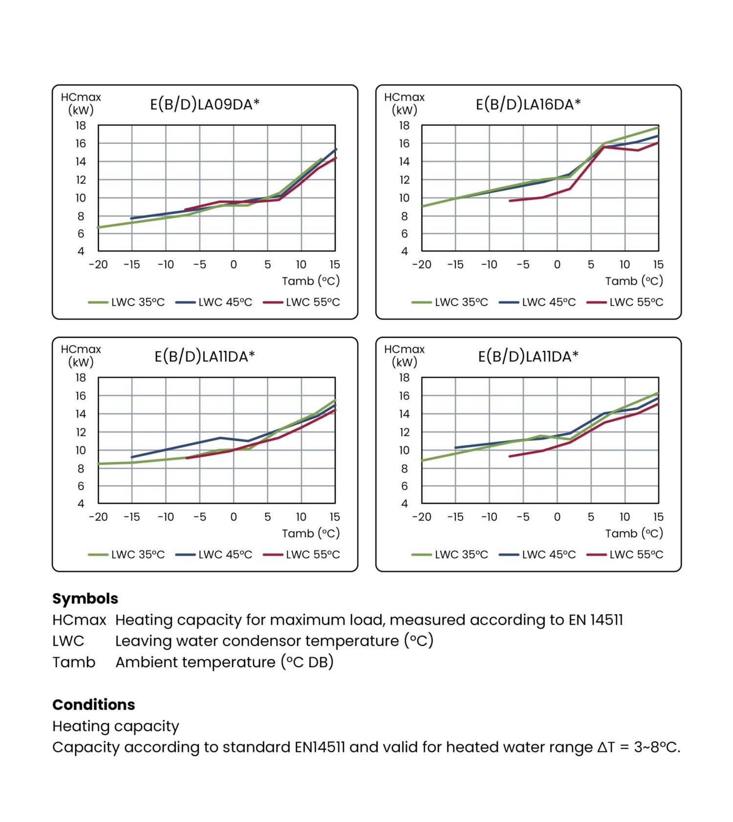
Some manufacturers display their information as graphs as well as, or instead of, tables as shown below. This visual representation can clarify the effect of both flow temperature and in this case ambient air temperature on the power output of the heat pump. It again shows us the impact of reduced ambient temperatures and increased system flow temperatures.
If you would like further information, contact the manufacturer’s local sales representative or technical support/presales helpline.
Maximum heating capacity – integrated value
Heat pump modulation
Most current heat pumps are inverter driven and can modulate their power output to match the heat load as it changes throughout the year. This varies from unit to unit with minimum power outputs ranging from 50-30%, with some producing as little as 12.5% of their rated maximum power output.
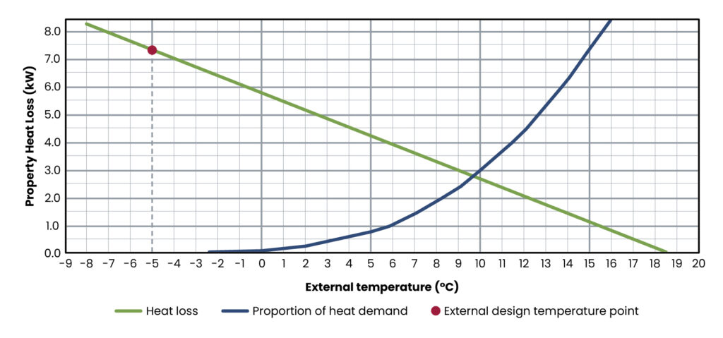
| Proportion of heating demand | External temp | Delta T | W/m² | Heating demand | ||
|---|---|---|---|---|---|---|
| °C | K | watts | kW | |||
| This shows the proportion of heating demand for each external temperature for a whole year. The heating percentage information is intended for guidance only acting as an approximation to provide property owners a better understanding of heating demands throughout a whole year. The amount of time the temperature falls below 2°C is only 3% of the year. 74% of the time the external temperatures are below 14°C. These averages are taken from the weather station at Gatwick airport over a 20 year average period (2002 to 2021). | 0.005% | -8 | 26.67 | 92.13 | 8267.75 | 8.27 |
| 0.01% | -7 | 25.67 | 88.67 | 7957.25 | 7.96 | |
| 0.02% | -6 | 24.67 | 85.22 | 7647.64 | 7.65 | |
| 0.04% | -5 | 23.67 | 81.76 | 7337.14 | 7.34 | |
| 0.09% | -4 | 22.67 | 78.31 | 7027.54 | 7.03 | |
| 0.18% | -3 | 21.67 | 74.86 | 6717.94 | 6.72 | |
| 0.35% | -2 | 20.67 | 71.4 | 6407.44 | 6.41 | |
| 0.65% | -1 | 19.67 | 67.95 | 6097.83 | 6.1 | |
| 1% | 0 | 18.67 | 64.49 | 5787.33 | 5.79 | |
| 2% | 1 | 17.67 | 61.04 | 5477.73 | 5.48 | |
| 3% | 2 | 16.67 | 57.58 | 5167.23 | 5.17 | |
| 5% | 3 | 15.67 | 54.13 | 4857.63 | 4.86 | |
| 7% | 4 | 14.67 | 50.68 | 4548.02 | 4.55 | |
| 9% | 5 | 13.67 | 47.22 | 4237.52 | 4.24 | |
| 12% | 6 | 12.67 | 43.77 | 3927.92 | 3.93 | |
| 17% | 7 | 11.67 | 40.31 | 3617.42 | 3.62 | |
| 22% | 8 | 10.67 | 36.86 | 3307.82 | 3.31 | |
| 28% | 9 | 9.67 | 33.4 | 2997.32 | 3 | |
| 35% | 10 | 8.67 | 29.95 | 2687.71 | 2.69 | |
| 43% | 11 | 7.67 | 26.49 | 2377.21 | 2.38 | |
| 52% | 12 | 6.67 | 23.04 | 2067.61 | 2.07 | |
| 63% | 13 | 5.67 | 19.59 | 1758.01 | 1.76 | |
| 74% | 14 | 4.67 | 16.13 | 1447.51 | 1.45 | |
| 87% | 15 | 3.67 | 12.68 | 1137.9 | 1.14 | |
| 100% | 16 | 2.67 | 9.22 | 827.4 | 0.83 | |
| CIBSE standard base temperature is 15.5% °C. Therefore, a buildings internal heat and solar gains contribute to the remaining demand above this temperature, so its assumed the heating system won't be in use. Only hot water will be required. | 17 | 1.67 | 5.77 | 517.8 | 0.52 | |
| 18 | 0.67 | 2.31 | 207.3 | 0.21 | ||
| 19 | -0.33 | -1.14 | -102.30 | -0.10 | ||
| 20 | -1.33 | -4.59 | -411.91 | -0.41 |
Source: Peter Emmerson, The Renewable Technology Collective
In this example we have a house with a heat demand of 7.34kW at -5°C DOT as the house is in Aberdeen.
If we use a design flow temperature of 45°C, we can look at the table above and see that 7kW will deliver a maximum of 8kW at -5°C with a flow temperature of 45°C.
| 35°C flow | 40°C flow | 45°C flow | 50°C flow | 55°C flow | |||||||
|---|---|---|---|---|---|---|---|---|---|---|---|
| Output | SCOP | Output | SCOP | Output | SCOP | Output | SCOP | Output | SCOP | ||
| 3.5kW | -5°C | 4.2 | 4.41 | 4.1 | 4.03 | 4 | 3.65 | 3.9 | 3.37 | 3.8 | 3.1 |
| -3°C | 4.6 | 4.4 | 4.3 | 4.2 | 4 | ||||||
| 0°C | 4.7 | 4.7 | 4.6 | 4.5 | 4.4 | ||||||
| 2°C | 4.9 | 4.9 | 4.9 | 4.7 | 4.6 | ||||||
| 5kW | -5°C | 6.3 | 4.48 | 6 | 4.13 | 5.6 | 3.77 | 5.5 | 3.41 | 5.4 | 3.06 |
| -3°C | 6.8 | 6.4 | 6.1 | 5.9 | 5.8 | ||||||
| 0°C | 6.9 | 6.7 | 6.6 | 6.4 | 6.2 | ||||||
| 2°C | 7.1 | 7 | 6.9 | 6.7 | 6.5 | ||||||
| 7kW | -5°C | 8.2 | 4.36 | 8.1 | 4.13 | 8 | 3.91 | 7.5 | 3.65 | 7 | 3.39 |
| -3°C | 8.8 | 8.6 | 8.4 | 7.9 | 7.4 | ||||||
| 0°C | 9.5 | 9.3 | 9.1 | 8.6 | 8.1 | ||||||
| 2°C | 10 | 9.8 | 9.6 | 9 | 8.5 | ||||||
| 10kW | -5°C | 9.9 | 5.03 | 9.7 | 4.58 | 9.4 | 4.13 | 9.1 | 3.85 | 8.8 | 3.58 |
| -3°C | 10.7 | 10.3 | 10 | 9.6 | 9.2 | ||||||
| 0°C | 11.9 | 11.6 | 11.3 | 10.7 | 10.2 | ||||||
| 2°C | 12.8 | 12.5 | 12.1 | 11.5 | 10.9 | ||||||
| 12kW | -5°C | 13.1 | 4.88 | 12.8 | 4.55 | 12.5 | 4.21 | 11.7 | 3.92 | 10.8 | 3.63 |
| -3°C | 13.9 | 13.4 | 12.9 | 12.1 | 11.2 | ||||||
| 0°C | 15.2 | 14.6 | 14.1 | 13.2 | 12.3 | ||||||
| 2°C | 16 | 15.5 | 14.9 | 13.9 | 13 | ||||||
Source: Vaillant “Be ready for the energy change”
This unit can modulate down to around 12.5% of its rated power output meaning that with careful installation and commissioning it should be able to run without significant cycling to around 15°C ambient air temperature.
Use excerpt from the data table above.
Single speed compressors, as used in legacy units (and some current commercial or specialist applications), require sufficient open volume or buffer storage to accommodate the surplus energy produced by a compressor designed to cover 100% of the heat load at the design temperature.
An inverter-driven unit’s minimum system volume is primarily intended to ensure sufficient heat energy is available to allow for an effective defrost cycle to be completed without adversely affecting the flow temperature of the system (see CIBSE domestic heating design guide section 1.6.5.8 page 44 CIBSE domestic heating design guide section for buffer sizing and manufacturer instructions for specific minimum available system volumes).
Six steps to ensure an accurately sized heat pump
- Carry out a room-by-room heat loss calculation as outlined in section 3.1 Heat loss calculations – detailed guidance.
- Decide on a design flow temperature at the DOT for the property’s location. (This may be in consultation with the customer or dependant on budget/practicalities of radiator oversizing and/or use of other emitter types).
- Select a heat pump that meets the needs of the project, including 100% of the heat demand of the house at the DOT. You may need to choose a unit with a slightly higher maximum power output if the heat load falls between two units maximum power output under those conditions.
- Verify the power output, additional efficiency data and installation requirements by using manufacturers’ data and, if required, by speaking to one of their representatives.
- Consider any site-specific reasons that may affect output and whether they can be mitigated without altering the unit selection.
- Attending manufacturer training for the range of units you are installing is recommended. Most have online learning modules designed to increase your familiarity with the unit before your first installation. Many also have free in-person training that will allow you to physically see the unit, its controls and understand any unique requirements specific to the heat pump you will be installing.